Introduction
When trading, success often hinges on having the right tools and understanding how to use them effectively. One such tool that has proven to be a popular classic is the Slow Stochastics indicator. This powerful technical analysis tool, with its unique ability to predict potential reversals in the market, has become a staple for many successful traders.
This indicator is a momentum oscillator that compares a security’s closing price to its price range over a specific period. It’s a variant of the original Stochastics indicator, developed by George C. Lane in the late 1950s, but with a twist – it uses a smoothing process to filter out market noise and deliver more accurate signals.
In this post, we’ll take a detailed exploration into the world of Slow Stochastics. We’ll have a look at its origins, its mathematical construction, and its purpose by design. We’ll also guide you on how to find buy and sell signals using this indicator, discuss its pros and cons, and even show you how to code it into your trading algorithms.
Whether you’re a novice trader just starting out or a seasoned pro looking to refresh your knowledge, this guide is designed to equip you with a thorough understanding of Slow Stochastics and how to leverage it for your trading success. So, let’s dive in and master the art of trading with Slow Stochastics.
Origins of Slow Stochastics
The Slow Stochastics indicator, as we know it today, is a modification of the original Stochastics oscillator, also now known as Fast Stochastics, which was developed by George C. Lane in the late 1950s. Lane, a renowned trader and a technical analysis innovator, introduced the Stochastics oscillator to help traders predict price turning points by comparing the closing price of a security to its price range over a specific period.
Lane believed that as prices increase, closing prices tend to be closer to the upper end of the price range, and as prices decrease, closing prices tend to be closer to the lower end of the price range. The Stochastics oscillator was designed to quantify this observation.
However, the original Stochastics oscillator was quite sensitive to market movements, often resulting in false signals. To mitigate this, traders introduced an additional smoothing process, creating what we now refer to as the Slow Stochastics. This smoothed version of the Stochastics oscillator reduces volatility and improves signal accuracy, making it a more reliable tool for traders.
| Fast Stochastics | Slow Stochastics | |
|---|---|---|
| Market Sensitivity | More sensitive to market movements | Less sensitive to market movements due to smoothing process |
| False Signals | Can result in more false signals | Can result in fewer false signals |
| Smoothing Process | Smoothing applied to %D line (3-day MA of %K) | Additional smoothing applied to both %K (which becomes Slow %K) and %D |
Mathematical Construction
The indicator consists of two lines:
- Slow %K Line: This line is similar to the %D line in the Fast Stochastics indicator. It’s calculated based on the closing price of a security relative to the range of its prices over a certain period.
- Slow %D Line: This line is a moving average of the Slow %K values. It helps smooth out the fluctuations in the Slow %K line to provide a clearer signal.
In the Fast Stochastics, the %D line is a 3-day simple moving average of the %K line, which is calculated directly from the price data. When transitioning to Slow Stochastics, this smoothed %D line from the Fast Stochastics becomes the Slow %K line. The Slow %D line is then derived as a 3-day simple moving average of this Slow %K line.
In essence, the Slow %K line in the Slow Stochastics is equivalent to the %D line in the Fast Stochastics. This transformation is done to smooth out the output and reduce the sensitivity to random price movements, hence providing more reliable trading signals.
Original Algorithm
The Original algorithm for calculating the Slow Stochastics indicator involves the following steps:
- Slow %K: Calculate the difference between the closing price and the lowest price in the lookback period. This gives you the closing range. Then, calculate the difference between the highest and lowest prices in the same period to get the total range. The ratio of the closing range to the total range is then smoothed using a moving average.
- Slow %D: Calculate the moving average of the Slow %K values.
The formulas for the Original algorithm are:
- K = (Moving Average (Close – Lowest Price, Smoothing Period, 3) / Moving Average (Highest Price – Lowest Price, Smoothing Period, 3)) * 100
- D = Moving Average ((Moving Average (Close – Lowest Price, Smoothing Period, 3) / Moving Average (Highest Price – Lowest Price, Smoothing Period, 3)), Smoothing Period, 3) * 100
Simplified Algorithm
The Simplified algorithm is more responsive to price changes and calculates the Slow Stochastics as follows:
- Slow %K: Calculate the ratio of the closing range to the total range first, and then apply the moving average.
- Slow %D: Calculate the moving average of the Slow %K values.
The formulas for the Simplified algorithm are:
- K = Moving Average ((Close – Lowest Price) / (Highest Price – Lowest Price), Smoothing Period, 3) * 100
- D = Moving Average (Moving Average ((Close – Lowest Price) / (Highest Price – Lowest Price), Smoothing Period, 3), Smoothing Period, 3) * 100
In both formulas, ‘Close’ is the closing price, ‘Lowest Price’ is the lowest price in the lookback period, ‘Highest Price’ is the highest price in the lookback period, and ‘Smoothing Period’ is the period used for smoothing the data. The ‘3’ in the formulas represents the period used for the moving average calculation in the Slow Stochastics indicator. The standard setting for Slow Stochastics is a 3-period average for this smoothing process, but this can be adjusted based on the trader’s preference.
Purpose by Design
The fundamental premise of this indicator is that in an upward trending market, closing prices are often near their peak, and conversely, in a downward trend, they’re near their lowest point.
The indicator is calculated by examining the relationship between a security’s closing price and its price range, which is defined by the highest and lowest prices during a specific period. This relationship is represented by the %K line. A smoothing process is then applied to the %K line, resulting in the %D line.
The interplay between the closing price and the price extremes of the period can significantly influence the indicator’s value. The values of the Slow Stochastics indicator can range from 0 to 100, typically represented as percentages. A value of 0% indicates that the closing price is equivalent to the lowest price during the specified period, while a value of 100% signifies that the closing price is the same as the highest price.
It’s important to note that these values are not absolute but are relative to the price range during the lookback period. This underscores the complexity of applying a linear calculation to a dataset that is inherently non-linear, such as price movements in a market.
There are two fundamental ways to interpret this indicator:
- The market is considered overbought when the indicator is above 80 and oversold when it’s below 20.
- Trading signals are generated when the lines cross within these extreme zones or have crossed and then exit these zones.
Another valuable application is as a divergence indicator. This is when the market reaches a new high, but the Stochastic doesn’t surpass its previous high and instead crosses downwards. This phenomenon is often referred to as a Failure Swing. The trading decision can be made either when the lines cross or exit the extremes.
However, it’s crucial to dispel some common misconceptions about the Slow Stochastics indicator. One such misconception is the profitability of the crossover theory. Empirical tests have shown that a crossover in an extreme zone can be unpredictable and potentially detrimental. The true value of Stochastics lies in the specific data it’s applied to, or the refined strategy it’s used in. Stochastics are most effective when used in markets that tend to revert to the mean. This is particularly relevant for spread or pairs trading on typically correlated stocks. Certain primary markets also exhibit a tendency for mean reversion.
Buy and Sell Signals
By interpreting the movements and crossovers of the Slow %K and Slow %D lines, traders can identify potential entry and exit points for their trades.
Overbought and Oversold Zones
One of the primary ways to use Slow Stochastics is to identify overbought and oversold conditions. When the Slow Stochastics value rises above 80, the market is typically considered overbought. Conversely, a value below 20 indicates an oversold market. These zones can signal potential price reversals, as markets often correct after reaching these extremes.
However, it’s important to note that markets can remain overbought or oversold for extended periods, especially during strong trends. Therefore, while these zones can provide valuable context, they should not be used as standalone signals.
Crossovers
Another common use of Slow Stochastics is to look for crossovers between the Slow %K and Slow %D lines. A bullish signal is generated when the Slow %K line crosses above the Slow %D line, and a bearish signal is generated when the Slow %K line crosses below the Slow %D line. These signals can be strengthened when they occur within the overbought or oversold zones.
As mentioned in the section above, consider the market where you would use this strategy, it is likely going to be more effective and less ruinous if using it for something like calendar spreads or pairs trading in stocks rather than markets prone to trend like commodities.
Divergences
Divergences between the Slow Stochastics indicator and the price action can also provide valuable trading signals. A bullish divergence occurs when the price forms a lower low, but the Slow Stochastics forms a higher low. This could indicate weakening downward momentum and a potential bullish reversal. Conversely, a bearish divergence occurs when the price forms a higher high, but the Slow Stochastics forms a lower high, indicating weakening upward momentum and a potential bearish reversal.
| Condition | Signal |
|---|---|
| Slow Stochastics > 80 | Market is overbought, potential sell signal |
| Slow Stochastics < 20 | Market is oversold, potential buy signal |
| %K line crosses %D line upwards | Bullish signal |
| %K line crosses %D line downwards | Bearish signal |
| Price forms a higher high, Stochastics forms a lower high | Bearish divergence, potential sell signal |
| Price forms a lower low, Stochastics forms a higher low | Bullish divergence, potential buy signal |
Best Stochastics Settings
The default setting is a 14-period lookback with a 3-period smoothing. However, these settings can be adjusted to better suit your trading style and the characteristics of the market you’re trading.
For short-term or day trading, you might consider reducing the lookback period to make the indicator more responsive to recent price changes. A setting of 5 or 7 periods could be more suitable in this case. However, keep in mind that a shorter lookback period will also make the indicator more sensitive to market noise, which could lead to more false signals.
For long-term trading or swing trading, a longer lookback period could be more appropriate. A setting of 21 or 28 periods could help filter out market noise and provide a clearer picture of the overall trend. However, a longer lookback period will also make the indicator less responsive to recent price changes.
The smoothing period can also be adjusted, but it’s generally recommended to keep this at 3 periods. A higher smoothing period will make the indicator less sensitive to market noise, but it will also make it less responsive to recent price changes.
Remember, there’s no “one size fits all” setting. The best settings will depend on your trading style, your risk tolerance, and the characteristics of the market you’re trading. It’s always a good idea to experiment with different settings and backtest your strategies before trading with real money.
Pros and Cons of the Slow Stochastics Indicator
Pros:
- Versatility: Slow Stochastics can be used in various ways, including identifying overbought and oversold conditions, generating trading signals through crossovers, and spotting divergences.
- Adaptability: It can be applied to any market (stocks, forex, commodities) and on any timeframe, making it a versatile tool for all types of traders.
- Complimentary signals: When used in conjunction with other technical analysis tools or indicators, Slow Stochastics can provide additional confirmation for trading signals, increasing the probability of successful trades.
Cons:
- Dodgy Signals in wrong markets: Slow Stochastics can produce false signals, especially in strongly trending markets where overbought and oversold conditions can persist for a long time. Particularly where looking at things like crossovers you are better off using that strategy in markets of a mean reverting nature (spread or stock pairs trading), as past studies have shown well under 50% accuracy of crossover signals in non mean reverting markets.
- Leading but with Caution: While Slow Stochastics is a leading indicator, it can sometimes provide premature signals, especially in volatile markets. This can result in potential false starts or early exits.
- Affected by Settings: The effectiveness of Slow Stochastics can greatly depend on the settings used. Incorrect settings can lead to misleading signals and potential losses, so you need to experiment and see what suits the timeframe and market you’re applying it to.
Coding and Charting Slow Stochastics with Python
Here’s a step-by-step guide to creating a Python script for calculating and plotting the Slow Stochastics indicator using VSCode (free software you can download from Microsoft). We’ll be going with the Simplified algorithm mentioned in the Mathematical Construction section for this example.
Step 1: Install the necessary Python libraries
Before you start writing the code, you need to make sure you have the necessary Python libraries installed. These libraries include yfinance for downloading stock data, pandas for data manipulation, mplfinance for financial data visualization, matplotlib for creating custom legends, and numpy for numerical operations.
You can install these libraries using pip, which is a package manager for Python. After setting up Python (you can follow the guide in VSCode to do that) open the terminal in VSCode (View -> Terminal) and type the following commands:
pip install yfinance pandas mplfinance matplotlib numpyStep 2: Import the necessary Python libraries
At the top of your Python script (save a new python file e.g slow_stochastics.py), you need to import the libraries that you will use. Each library has a specific purpose:
import yfinance as yf
import pandas as pd
import mplfinance as mpf
import matplotlib.pyplot as plt
from matplotlib.lines import Line2D
import numpy as np
Step 3: Define the function to calculate Slow Stochastics
Next, you need to define a function that calculates the Slow Stochastics. This function takes as input the security’s data and a lookback period, and returns the Slow %K and Slow %D lines. The lookback period is the number of trading days or periods used for the calculation. For shorter time trading horizons, you might want to decrease this number, which you can do in Step 5 below.
def calculate_slow_stochastics(data, lookback):
    low_min  = data['Low'].rolling( window = lookback ).min()
    high_max = data['High'].rolling( window = lookback ).max()
    k = 100 * (data['Close'] - low_min) / (high_max - low_min)
    d = k.rolling(window = 3).mean()
    return k, d
This function is more aligned with the Simplified Algorithm mentioned in the Mathematical Construction section of this post, where the calculation is done prior to smoothing.
Step 4: Download the stock data
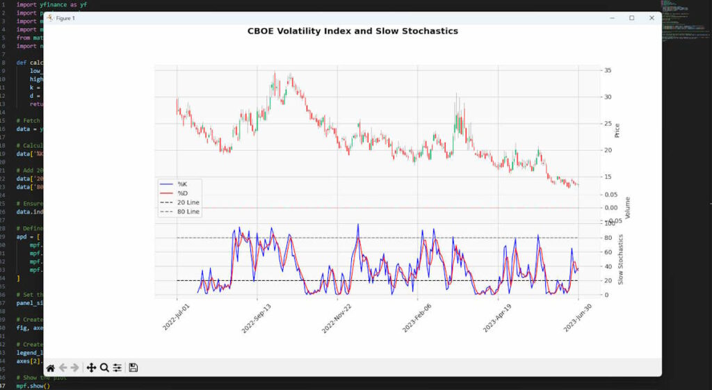
You can download the stock data using the yfinance library. In this case, we are downloading data for the CBOE Volatility Index (^VIX) from July 1, 2022, to July 1, 2023. If you want to analyze a different security or time period, you can change the ticker symbol and dates.
data = yf.download('^VIX', start='2022-07-01', end='2023-07-01')Step 5: Calculate the Slow Stochastics
You can now calculate the Slow Stochastics by calling the function you defined earlier. The calculated values are added as new columns to the stock data.
data['%K'], data['%D'] = calculate_slow_stochastics(data, 14)Step 6: Add the 20 and 80 lines
The Slow Stochastics indicator is typically used with two threshold lines at 20 and 80. Signals are generated when the %K line crosses these threshold lines. You can add these lines as new columns to the stock data.
data['20 Line'] = 20
data['80 Line'] = 80
Step 7: Ensure the index is a DatetimeIndex
The mplfinance library requires the index of the stock data to be a DatetimeIndex. You can ensure this with the following line of code:
data.index = pd.DatetimeIndex(data.index)Step 8: Define the additional plots
You can define the additional plots (Slow %K, Slow %D, 20 line, 80 line) as a list of dictionaries. Each plot is created using the mpf.make_addplot function, which takes as input the data to be plotted, the panel where the plot should be displayed, the color of the plot, whether the plot should use a secondary y-axis, and the linestyle.
apd = [
    mpf.make_addplot(data['%K'], panel=2, color='b', secondary_y=False, ylabel='Slow Stochastics'),
    mpf.make_addplot(data['%D'], panel=2, color='r', secondary_y=False),
    mpf.make_addplot(data['20 Line'], panel=2, color='black', secondary_y=False, linestyle='dashed'),
    mpf.make_addplot(data['80 Line'], panel=2, color='grey', secondary_y=False, linestyle='dashed')
]
Step 9: Set the panel sizes
You can set the sizes of the panels using the panel_ratios parameter. In this case, the first panel (candles) is set to 5 and the second and third panels (volume and Slow Stochastics) 1 and 3 respectively.
panel_sizes = (5, 1, 3)Step 10: Create the plot
You can now create the plot using the mpf.plot function. This function takes as input the stock data, the type of plot (candle), the style of the plot, the additional plots, whether to include volume, the panel sizes, the title of the plot, and whether to return the figure and axes.
fig, axes = mpf.plot(data, type='candle', style='yahoo', addplot=apd, volume=True, panel_ratios=panel_sizes, title='CBOE Volatility Index and Slow Stochastics', returnfig=True)Step 11: Create the legend
You can create a custom legend using dummy lines. The legend lines are created using the Line2D class from matplotlib, and the legend is added to the plot using the legend method.
legend_lines = [Line2D([0], [0], color=c, lw=1.5, linestyle=ls) for c, ls in zip(['b', 'r', 'black', 'grey'], ['solid', 'solid', 'dashed', 'dashed'])]
axes[2].legend(legend_lines, ['%K', '%D', '20 Line', '80 Line'], loc='lower left')
Step 12: Show the plot
Finally, you can display the plot using the mpf.show function.
mpf.show()Step 13: Run the script
You can run the script by clicking on the “Run” button in the top right corner of VSCode or by pressing F5. If everything is set up correctly, you should see a plot of the CBOE Volatility Index with the Slow Stochastics indicator.
Remember to save your script with a .py extension (for example, slow_stochastics.py) before running it. If you encounter any errors, make sure you have installed all the necessary libraries and that the code is written correctly.
If all has gone to plan you will end up with a chart looking like the one I made below:

You could go on to develop this code as part of a stochastics screener, probably combined with other indicators and have it alert you to charts you wouldn’t normally have space to be analysing constantly.
Key Takeaways
- The Slow Stochastics indicator is a variation of the original Fast Stochastics, both developed by George Lane. The key difference is the additional smoothing applied in Slow Stochastics to reduce sensitivity to market noise.
- The indicator is calculated using the closing price of a security relative to its price range over a specific period, represented by the %K line. A smoothing process is then applied, forming the %D line.
- It’s versatile, with applications in identifying overbought and oversold conditions, generating trading signals through crossovers, and spotting divergences.
- The indicator’s values range from 0 to 100, with values above 80 typically indicating overbought conditions and values below 20 indicating oversold conditions.
- Despite its utility and being considered as a leading indicator, it can produce false signals, especially in strongly trending markets.
- The effectiveness of the indicator can greatly depend on the settings used. The default setting is a 14-period lookback with a 3-period smoothing, but these can be adjusted to better suit different trading styles and market conditions.
- The Slow Stochastics indicator is most effective when used in markets that tend to revert to the mean, such as spread or pairs trading on typically correlated stocks. Certain primary markets also exhibit a tendency for mean reversion.
- Traders can code this indicator into their trading algorithms to automate the generation of trading signals. We presented a guide of how to get started with it in Python in this post’s step by step guide.


Leave a Reply