
Introduction
The Average True Range (ATR) is a technical analysis indicator that measures market volatility by decomposing the entire range of an asset price for that period. It was developed by J. Welles Wilder Jr., a mechanical engineer and real estate developer, who also created other popular technical analysis indicators like the Relative Strength Index (RSI) and the Parabolic SAR.
The ATR itself is an absolute value, usually measured in the currency or points of the particular market. The average true range percent (ATR%) is a relative measure of the ATR, expressing the ATR as a percentage of the closing price. This makes the ATR% a dimensionless quantity, allowing it to be compared across different price levels and instruments.
Mathematical Construction
This indicator is calculated using the true range of the asset price, which is defined as the greatest of the following:
- The current high less the current low.
- The absolute value of the current high less the previous close.
- The absolute value of the current low less the previous close.
Let’s break down these three components:
- Current High less the Current Low: This is simply the range of the current trading period (day, hour, etc.). It represents the distance between the highest and lowest prices during the period.
- Absolute Value of (Current High less the Previous Close): This measures the distance from the current high to the previous close. If the current high is greater than the previous close (indicating a gap up or an upward movement), this will be a positive value. If the current high is less than the previous close (indicating a gap down or a downward movement), this will be a negative value. Taking the absolute value ensures that we are always dealing with a positive distance.
- Absolute Value of (Current Low less the Previous Close): This measures the distance from the current low to the previous close. Again, taking the absolute value ensures that we are always dealing with a positive distance.
The True Range is the greatest of these three values. This ensures that the True Range takes into account any significant gap from the close of the previous period to the high or low of the current period.
| Period | Current High | Current Low | Previous Close | Current High – Current Low | Absolute Value of (Current High – Previous Close) | Absolute Value of (Current Low – Previous Close) | True Range |
|---|---|---|---|---|---|---|---|
| 1 | H1 | L1 | C0 | H1 – L1 | abs(H1 – C0) | abs(L1 – C0) | TR1 |
| 2 | H2 | L2 | C1 | H2 – L2 | abs(H2 – C1) | abs(L2 – C1) | TR2 |
| … | … | … | … | … | … | … | … |
| n | Hn | Ln | C(n-1) | Hn – Ln | abs(Hn – C(n-1)) | abs(Ln – C(n-1)) | TRn |
The table above provides a detailed breakdown of the calculations involved in determining the True Range for each period, a fundamental step in calculating the indicator’s value. Each row of the table represents a specific trading period, displaying the values for the Current High, Current Low, and Previous Close, along with the calculations required to compute the True Range.
- Current High – Current Low: This column illustrates the range of the current trading period, representing the distance between the highest and lowest prices during that period.
- Absolute Value of (Current High – Previous Close): This column measures the absolute distance from the current high to the previous close, ensuring that any gap up or downward movement is accounted for as a positive distance.
- Absolute Value of (Current Low – Previous Close): Similar to the previous column, this one measures the absolute distance from the current low to the previous close, also ensuring a positive distance.
- True Range: The final column represents the True Range, which is the greatest value among the three calculated in the preceding columns. This ensures that the True Range takes into account any significant gap from the close of the previous period to the high or low of the current period.
Understanding the True Range is essential to grasping how the ATR is subsequently calculated, as it forms the basis for the exponential moving average calculation used to determine the ATR according to Wilder’s method.
Wilder’s method refers to the exponential smoothing technique used. Unlike a simple moving average that weighs all data points equally, Wilder’s method of using an EMA places greater weight on recent data. This method is particularly suited for this calculation as it helps in reflecting recent market volatility more responsively. It is often used with a smoothing constant determined by the period, such as 1/n, where n is the number of periods over which the ATR is calculated.
So the Average True Range (ATR) is then calculated by taking an exponential moving average of the True Range over a specified number of periods. For example, a 14-day ATR would calculate the average True Range over the past 14 days. This gives a measure of volatility that smooths out single-day spikes and troughs, providing a more consistent and reliable measure of market volatility.
The formula is as follows:
ATR = ((1 – (1 / n)) * Previous ATR) + ((1 / n) * Current True Range)
which is the same as:
\text{{ATR}} = \left(1 - \frac{1}{n}\right) \times \text{{Previous ATR}} + \frac{1}{n} \times \text{{Current True Range}}
where:
- n is the period you want to calculate the ATR over (for example, if you want to calculate the ATR over a 14-day period, n would be 14).
- Previous ATR is the ATR value from the previous period.
- Current True Range is the true range for the current period.
The indicator is typically calculated using daily data, but it can also be used with any time frame (like hourly, weekly, or monthly data).
Average True Range Percent (ATR%)
Another variation of this that traders often utilize is the Average True Range Percent (ATR%). As I mentioned in the introduction while the ATR provides an absolute measure of volatility, the ATR% gives a relative perspective by expressing the ATR as a percentage of the current price level.
The formula is:
ATR% = (ATR / Current Price) * 100
which is the same as:
\text{{ATR\%}} = \left(\frac{{\text{{ATR}}}}{{\text{{Current Price}}}}\right) \times 100
It can be particularly useful when comparing the volatility of assets with significantly different price levels. By expressing the ATR as a percentage, it provides a normalized view of volatility, allowing for a more meaningful comparison.
Purpose and Use
The ATR is primarily used to measure volatility. It does not provide any indication of price direction or trend. It simply quantifies the degree of price volatility. This is useful for traders because high volatility often occurs at market turning points, and low volatility often occurs during normal market conditions. By helping to distinguish between these two scenarios, the indicator can help traders to manage their trades more effectively.
It can also be used to set stop loss levels. A common strategy is to set the stop loss at a multiple of the ATR. For example, a trader might set the stop loss at twice its value. This means that if the ATR is 0.5, the stop loss would be set at 1.0. This strategy helps to ensure that the stop loss is set at a level that is appropriate for the current market conditions.
How to Interpret Signals
This indictor is a measure of market volatility. High values indicate high volatility and large price ranges, while low values indicate low volatility and small price ranges.
It does not indicate price direction, only volatility. Therefore, a rising value indicates increasing volatility regardless of whether prices are rising or falling. Similarly, a falling ATR indicates decreasing volatility whether prices are moving up or down.
Traders often use the it to adjust their trading strategies according to the market’s volatility. For example, in a high volatility market, traders might widen their stop loss and take profit levels to avoid being stopped out of a trade due to a sudden price swing. In a low volatility market, traders might tighten their stop loss and take profit levels to capture profits more quickly and protect against sudden price reversals.
Pros and Cons
Like all technical indicators, this one also has its strengths and weaknesses.
Pros:
- Versatility: It can be used in all markets, including stocks, forex, commodities, and futures, and on any timeframe, from intraday charts to monthly charts.
- Adaptability: It automatically adjusts to changes in volatility, making it a dynamic and adaptable tool for traders.
- Risk Management: The ATR can be used to set stop loss levels that are proportional to the current market volatility, helping traders to manage their risk more effectively.
Cons:
- No Directional Information: The indicator only measures volatility, not price direction. It needs to be used in conjunction with other indicators or analysis techniques to determine the direction of the trend.
- Lagging Indicator: Like all indicators based on past price data, it is a lagging indicator. It reflects past volatility, not future volatility. While it can help traders to adapt to changes in volatility, it cannot predict those changes.
- It Ignores Fundamentals Further to the point made above, if you happen to be waiting for a big event to occur later in the week such as an earnings announcement, an interest rate decision or something like non-farm payrolls then I find using something like ATR is not helpful for placing stops. This is because the range will shrink in quiet markets awaiting what will likely be a huge move at the time of the upcoming event. Always think about the wider market context, don’t get buried in binary interpretations of indicator outputs.
Coding it
The ATR can be coded into a trading algorithm using various programming languages. Here’s an example of how to calculate it in Python using the pandas library, in accordance with the method by Wilder:
import pandas as pd

def calculate_atr(data, period):
    high_low = data['High'] - data['Low']
    high_close = (data['High'] - data['Close'].shift()).abs()
    low_close = (data['Low'] - data['Close'].shift()).abs()

    ranges = pd.concat([high_low, high_close, low_close], axis=1)
    true_range = ranges.max(axis=1)

    # Initializing ATR with the average of the first 'period' True Range values
    atr = pd.Series(index=true_range.index)
    atr.iloc[0:period] = true_range.iloc[0:period].mean()

    # Calculating ATR using Wilder's exponential smoothing method
    for i in range(period, len(atr)):
        atr.iloc[i] = ((1 - (1 / period)) * atr.iloc[i - 1]) + ((1 / period) * true_range.iloc[i])

    return atr
In this code, data is a DataFrame that contains the high, low, and close prices for each period, and period is the number of periods over which to calculate the ATR. The function first calculates the three components of the True Range, then finds the maximum of these three values for each period to get the True Range. The ATR is then calculated using an exponential smoothing method over the specified number of periods, following Wilder’s original approach.
The equivalent code in R for the above would be:
calculate_atr <- function(data, period) {
  high_low <- data$High - data$Low
  high_close <- abs(data$High - lag(data$Close))
  low_close <- abs(data$Low - lag(data$Close))

  true_range <- pmax(high_low, high_close, low_close, na.rm = TRUE)

  # Initialize ATR with the average of the first 'period' True Range values
  atr <- numeric(length(true_range))
  atr[1:period] <- mean(true_range[1:period], na.rm = TRUE)

  # Calculate ATR using Wilder's exponential smoothing method
  for (i in (period + 1):length(atr)) {
    atr[i] <- ((1 - (1 / period)) * atr[i - 1]) + ((1 / period) * true_range[i])
  }

  return(atr)
}

# Example usage:
# data <- data.frame(High = c(...), Low = c(...), Close = c(...))
# period <- 14
# atr <- calculate_atr(data, period)
Plotting it with Python
Below I will offer a step-by-step guide to creating a Python script in VS Code. Use ‘pip install’ to first install the necessary libraries after installing Python (posts on other indicators I’ve written give greater detail how to do this if you’re uncertain but it’s the same process). This script will download some stock data, calculate the Average True Range (ATR) and ATR% for the specified period, and then plot it all together.
So create your .py file and start adding the code parts below to it in the same order.
Step 1: Import Necessary Libraries
import yfinance as yf
import pandas as pd
import mplfinance as mpf
import matplotlib.pyplot as plt
from matplotlib.lines import Line2D
Above, you are importing the necessary libraries to fetch stock data, manipulate it, and visualize it.
Step 2: Define Functions for Calculating ATR and ATR%
def calculate_atr(data, period):
    high_low = data['High'] - data['Low']
    high_close = (data['High'] - data['Close'].shift()).abs()
    low_close = (data['Low'] - data['Close'].shift()).abs()

    ranges = pd.concat([high_low, high_close, low_close], axis=1)
    true_range = ranges.max(axis=1)

    # Initializing ATR with the average of the first 'period' True Range values
    atr = pd.Series(index=true_range.index)
    atr.iloc[0:period] = true_range.iloc[0:period].mean()

    # Calculating ATR using Wilder's exponential smoothing method
    for i in range(period, len(atr)):
        atr.iloc[i] = ((1 - (1 / period)) * atr.iloc[i - 1]) + ((1 / period) * true_range.iloc[i])

    return atr

def calculate_atr_percent(data, atr):
    return (atr / data['Close']) * 100
Step 3: Download Data and Calculate ATR and ATR%
data = yf.download('META', start='2022-08-03', end='2023-08-03')
period = 14
atr = calculate_atr(data, period)
data['ATR'] = atr
data['ATR%'] = calculate_atr_percent(data, atr)
Step 4: Define Additional Plots and Panel Sizes
apd = [
    mpf.make_addplot(data['ATR'], panel=2, color='g', ylabel='ATR'),
    mpf.make_addplot(data['ATR%'], panel=3, color='r', ylabel='ATR%')
]
panel_sizes = (5, 1, 3, 3)
Step 5: Create the Plot and Customize the Appearance
fig, axes = mpf.plot(data, type='candle', style='yahoo', addplot=apd, volume=True, panel_ratios=panel_sizes, title='Meta Platforms Inc.', returnfig=True)

# Add a thin frame around each panel
for ax in axes:
    for spine in ax.spines.values():
        spine.set_edgecolor('black')
        spine.set_linewidth(0.5)

# Dummy lines for custom legends
legend_lines = [Line2D([0], [0], color='g', lw=2), Line2D([0], [0], color='r', lw=2)]
fig.legend(legend_lines, ['ATR', 'ATR%'], bbox_to_anchor=(0.05, 0.5), loc='center left', frameon=False)

plt.show()
In this step, you create the plot using the mplfinance library, add a thin frame around each panel, create custom legends, and display the plot.
So finally you would save the file and press the play button in the top right to execute the script which will then produce a chart like mine shown below. You can double check it with something like Yahoo Finance charts using their 14 period ATR with the same dates and you’ll see our green line is identical, which is always reassuring.
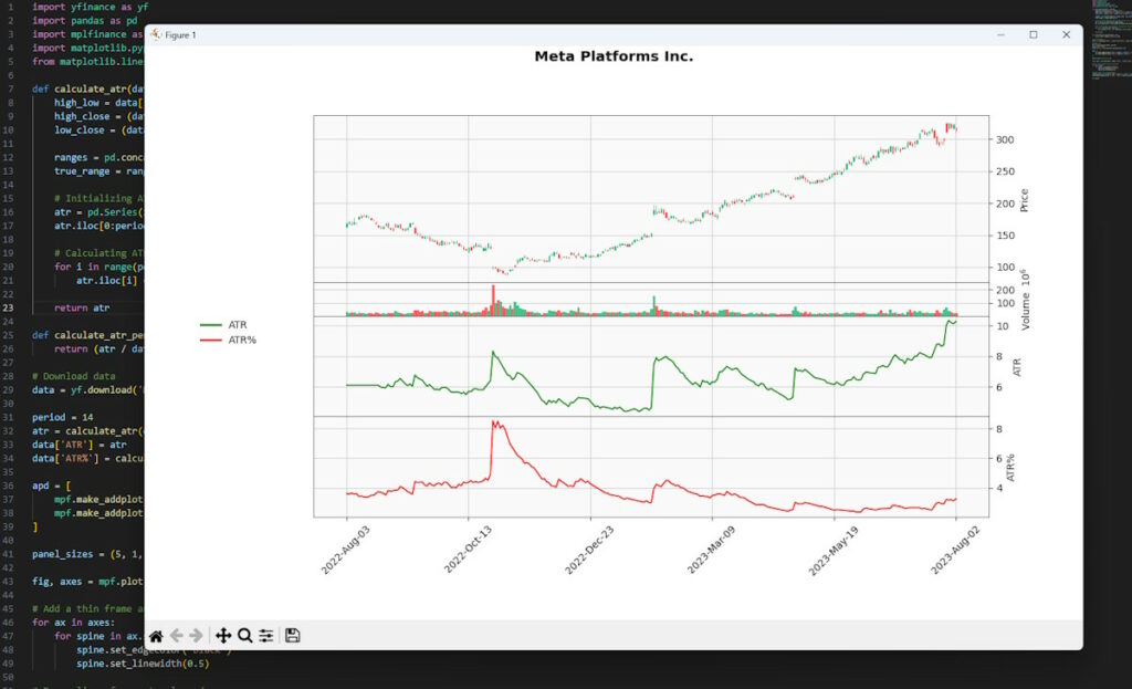
The average true range percentage (ATR%) shown here is not calculated as a percentage of the total range over the past 14 days. Instead, it is calculated as a percentage of the closing price. This allows the ATR% to be compared across different price levels and instruments, providing a dimensionless quantity that represents volatility relative to the current price.
A Different Average True Range Percent Approach
If you should want to calculate the percentage of the current day’s true range relative to the average of the past 14 days’ true ranges (i.e., the ATR), you would need a different calculation. Here’s how you would it:
def calculate_true_range_percent(data, atr):
    true_range_percent = []
    for i in range(len(data)):
        true_range_current = max(data['High'].iloc[i] - data['Low'].iloc[i],
                                abs(data['High'].iloc[i] - data['Close'].iloc[i - 1]),
                                abs(data['Low'].iloc[i] - data['Close'].iloc[i - 1])) if i > 0 else 0
        atr_current = atr.iloc[i]
        true_range_percent.append((true_range_current / atr_current) * 100 if atr_current != 0 else 0)
    return pd.Series(true_range_percent, index=data.index)
You can call this function with your data and ATR to get the percentage of the current day’s true range relative to it.
data['ATR%'] = calculate_true_range_percent(data, atr)If there’s a market gap, this percentage might be several hundred percent.
So after plugging that into our code and generating the chart we now get it as the modified red line:
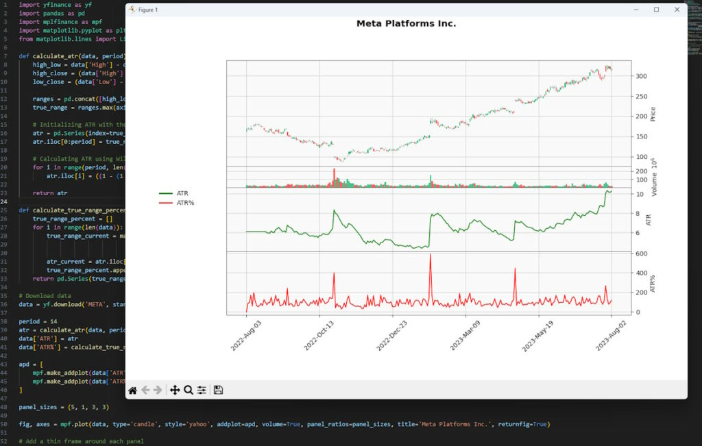
This then provides a percentage visual guide of the range breaking out. This would typically be caused by the market awaiting say, earning releases for the stock and the market absorbing that after hours creating big gaps when it opens again.
Clarification of Our Two Different ATR% Calculations
| Calculation Method | Formula | Usage Description |
|---|---|---|
| ATR% as a Percentage of Closing Price | ATR% = (ATR / Current Price) × 100 | Normalizes the ATR by expressing it as a percentage of the current price level, allowing for comparisons of volatility across different assets or timeframes. |
| ATR% Relative to the Lookback Period (True Range Percent) | True Range Percent = (Current True Range / ATR) × 100 | Provides insight into how the current day’s range compares to recent historical volatility, useful for detecting breakouts or sudden changes in volatility. |
Practical Examples
To understand the practical application of the ATR, let’s consider a few real-world examples.
Example 1: Setting Stop Loss Levels
Suppose you’re trading a stock that’s currently priced at $100. The 14-day ATR is 2. This means that, on average, the stock has moved $2 per day over the past 14 days. To set a stop loss that’s 2 times the ATR, you would set it $4 below the current price, or at $96. This gives the stock enough room to move in its normal range without hitting your stop loss, while still protecting you from a significant adverse move.
Example 2: Identifying Market Changes
Suppose you’re trading a forex pair, and you notice that the ATR has been steadily increasing over the past few days. This indicates that the market is becoming more volatile. As a result, you might decide to trade smaller position sizes to manage your risk, or you might look for trading strategies that perform well in volatile markets.
Comparison with Other Indicators
This is a unique indicator in that it measures volatility, not price direction. However, it can be compared to other volatility indicators.
For example, the Bollinger Bands indicator also measures volatility. The width of the Bollinger Bands is a measure of volatility, with wider bands indicating higher volatility and narrower bands indicating lower volatility. However, unlike the ATR, Bollinger Bands also provide information about price direction and overbought/oversold conditions.
Another volatility indicator is the Standard Deviation, which measures the dispersion of a dataset relative to its mean. The higher the standard deviation, the greater the volatility. However, standard deviation assumes a normal distribution of data, which is not always the case in financial markets.
Conclusion
Understanding market volatility is essential for traders, and the tool discussed in this post offers a dynamic way to gauge it. Applicable across various markets and timeframes, this indicator can be a versatile part of a trader’s strategy. Though it doesn’t offer insights into price direction, when combined with other analytical methods, it can aid in risk management, trade optimization, and recognizing potential market shifts.
Key Takeaways:
- Versatility: Suitable for stocks, forex, commodities, and futures, and adaptable to different timeframes.
- Risk Management: Useful in setting stop loss levels proportional to current market conditions.
- Interpretation: Provides valuable information on volatility but must be used with other indicators to understand price trends.
- Real-World Applications: Practical in various trading scenarios, from setting stop loss levels to identifying market changes.
- Comprehensive Analysis: A reminder that relying solely on one indicator may lead to incomplete decision-making. Combining various tools and techniques enhances trading accuracy and success.
- Fundamental Consideration: While the indicator provides insights into historical volatility, it may not adequately account for fundamental market events that can drastically affect price movements. Ignoring such events and placing stops based solely on tight preceding ranges can lead to unexpected losses, especially if the market is awaiting significant news like earnings announcements or interest rate decisions. You can see this on our second chart of the modified average true range percent spikes being several hundred percent. Integrating a broader understanding of market context ensures a more robust and responsive trading strategy.
Further Reading
Wilder, J. Welles. “New Concepts in Technical Trading Systems.” Trend Research, 1978.



Leave a Reply