Fast Stochastics: Best Stochastics Settings and Code

Table of Contents

Introduction

Fast Stochastics is a popular momentum indicator used in technical analysis to help traders predict price trends. It’s particularly useful for identifying potential overbought and oversold conditions in the market. The indicator is based on the premise that as a market trends upward, prices will close near their high, and as a market trends downward, prices will close near their low.

Origins

The Fast Stochastics indicator was first introduced by George C. Lane in the 1950s and represents the original version of the stochastics indicator. Over time, to cater to different trading preferences, a variation known as Slow Stochastics was developed, which incorporates additional smoothing techniques. The primary aim of the Fast Stochastics indicator was to enhance trading performance by pinpointing significant price trends and potential turning points. Due to its efficacy in providing a swift snapshot of market momentum, it has become an indispensable tool for many traders.

While the Fast Stochastics does involve a degree of smoothing (typically seen in the calculation of the %D line), the Slow Stochastics variation incorporates an additional layer of smoothing. This added smoothing in Slow Stochastics is applied to both the %K and %D lines, making it less sensitive to daily price fluctuations and often preferred for longer-term analysis. I’ve written about the nuances of the Slow Stochastics in another dedicated post.

Mathematical Construction of Fast Stochastics

The Fast Stochastics indicator is calculated using a two-step process. The first step involves calculating the Fast %K value. This is done by identifying the highest high, lowest low, and the current price for a specified period. The lowest low is subtracted from the current price, and then the difference is divided by the range (where the range is the highest high – lowest low). This result becomes the first Fast %K value.

The system continues to calculate Fast %K values by excluding the oldest bar and including the next more recent bar before repeating the above calculation.

The second step involves calculating the Fast %D value, which is a moving average of Fast %K values. The default for Fast %D is a smoothed 3-period moving average.

Here’s a detailed breakdown of each component and the formula used to calculate them:

Fast %K

Fast %K is the main line of the Fast Stochastics indicator. It’s calculated using the following formula:

Fast %K = [(Close – Lowest Low) / (Highest High – Lowest Low)] * 100

which can also be show as:

\text{Fast \%K} = \left( \frac{\text{Close} - \text{Lowest Low}}{\text{Highest High} - \text{Lowest Low}} \right) \times 100

Where:

Term	Definition
Close	The closing price of the current period.
Lowest Low	The lowest price traded during a specified number of periods.
Highest High	The highest price traded during the same number of periods.

Formula components explained

This formula essentially measures the closing price in relation to the range of prices over a specified period. The result is then multiplied by 100 to create a percentage.

Fast %D

Fast %D is a moving average of Fast %K values. It’s calculated using the following formula:

\text{Fast \%D} = \text{3-period moving average of Fast \%K}

The default for Fast %D is a smoothed 3-period moving average, but this can be adjusted based on the trader’s preference.

These two lines (%K and %D) are plotted on a scale from 0 to 100, with lines drawn at the 20 and 80 levels to create a signal or trigger line. When the Fast %K line crosses above the Fast %D line, it generates a buy signal, and when it crosses below the Fast %D line, it generates a sell signal.

Best Stochastics Settings

The Stochastics indicator, can be tailored through its settings to fit various trading strategies and market conditions. Knowing the optimal settings for your specific trading goals is crucial for maximizing the efficacy of the indicator.

1. Default Settings:

The most commonly used and default setting for the Fast Stochastics is a 14-period lookback for %K and a 3-period moving average for %D. The default 14-period lookback setting is based on the idea that a two-week span effectively captures price momentum and trends However, it’s essential to note that these settings might not be optimal for all market conditions or trading strategies.

2. Alternative Settings:

Adjusting the settings can provide a different perspective on price momentum and potential trend reversals:

Shorter Periods: Some traders prefer shorter periods, such as a 5 or 9-period lookback for %K, especially for more volatile markets or short-term trading strategies. These settings can produce more frequent trading signals but may also increase the risk of false signals.
Longer Periods: For traders with a longer-term perspective or for less volatile markets, extending the lookback period, say to 21 or 28 periods, might be beneficial. This approach can provide a smoother line and fewer, but potentially more reliable, signals.

3. Impacts of Adjusting Settings:

Modifying the settings will invariably affect the behaviour of the Stochastics lines:

Increased Sensitivity: Shortening the lookback period can make the Stochastics more responsive to price changes, which may be useful in rapidly moving markets. However, this increased sensitivity can also lead to more false signals.
Decreased Sensitivity: Lengthening the lookback period can reduce the indicator’s sensitivity, providing a clearer picture of more prolonged trends. While this might reduce the number of false signals, it can also result in slower reactions to genuine trend reversals.

While the default settings are a great starting point, adjusting the Stochastics settings to align with your trading strategy and the specific market you’re trading in is key. It’s always recommended to backtest different settings on historical data before implementing them in live trading.

Purpose and Design of Fast Stochastics

The Fast Stochastics indicator measures the closing price of a security relative to the high-low range over a given period of time. By doing so, it helps traders predict potential reversal points in the market, as the indicator tends to make a turn before the price does. This characteristic makes it a leading indicator in technical analysis.

Interpreting Fast Stochastics Signals

Interpreting the Fast Stochastics indicator involves understanding the relationship between the Fast %K and Fast %D lines. When the Fast %K line crosses above the Fast %D line, it generates a buy signal, indicating that it might be a good time to enter a long position. Alternatively, when the Fast %K line crosses below the Fast %D line, it generates a sell signal, suggesting that it might be a good time to exit a long position or enter a short position.

Fast %K Movement	Signal Generated
Crosses above Fast %D	Buy
Crosses below Fast %D	Sell

Conditions for buy and sell signals to appear

In addition, the Fast Stochastics indicator is also used to identify overbought and oversold conditions. Generally, a value above 80 is considered overbought, suggesting that a price might be nearing a top and could be due for a reversal. On the other hand, a value below 20 is considered oversold, indicating that a price might be nearing a bottom and could be due for a bounce.

Fast Stochastics Value	Market Condition
Above 80	Overbought
Below 20	Oversold

How overbought and oversold conditions are generally determined

Pros and Cons

Like any technical analysis tool, this indicator also has its strengths and weaknesses. One of the main advantages of using the Fast Stochastics indicator is its ability to identify potential price reversals ahead of time. This can give traders a valuable head start, allowing them to position themselves accordingly before the price moves.

However, it also has its limitations. For instance, it can produce false signals during periods of sideways or range-bound market activity. This is because the indicator is designed to work best in trending markets, and its performance can suffer during periods of low volatility.

Coding Fast Stochastics in Popular Trading Languages

Coding this indicator into popular trading languages like Python or R can provide traders with a greater degree of flexibility and control over their trading strategies. Here’s a basic example of how you might code the Fast Stochastics indicator in Python using the pandas library:

Python

import pandas as pd

# Define the lookback period
lookback = 14

# Define the smoothing period for %D
smooth_period = 3

# Calculate the highest high and lowest low over the lookback period
high = df['High'].rolling(window=lookback).max()
low = df['Low'].rolling(window=lookback).min()

# Calculate Fast %K
df['%K'] = (df['Close'] - low) / (high - low) * 100

# Calculate Fast %D
df['%D'] = df['%K'].rolling(window=smooth_period).mean()

In this code snippet, df is a DataFrame that contains the high, low, and close prices for a given security. The %K and %D values are then calculated and added as new columns to the DataFrame.

Here’s an example of how you might code the Fast Stochastics indicator in R using the quantmod and TTR libraries where we first install and load the quantmod and TTR libraries. We then download the historical data for Alibaba using the getSymbols function from the quantmod library. The stoch function from the TTR library is used to calculate Fast %K and Fast %D. The results are added as new columns to the data frame:

# Install necessary libraries
install.packages(c("quantmod", "TTR"))

# Load the libraries
library(quantmod)
library(TTR)

# Download historical data for Alibaba
getSymbols("BABA", src = "yahoo", from = "2022-01-01", to = Sys.Date())

# Define the lookback period
lookback <- 14

# Calculate Fast %K
BABA$fastK <- stoch(BABA[,c("BABA.High","BABA.Low","BABA.Close")], n=lookback, fastK=1, fastD=3)$fastK

# Calculate Fast %D
BABA$fastD <- stoch(BABA[,c("BABA.High","BABA.Low","BABA.Close")], n=lookback, fastK=1, fastD=3)$fastD

# Print the data
print(head(BABA))

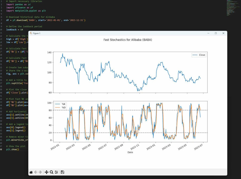
Here’s an example of how you might use Python and the matplotlib library to plot the Fast Stochastics indicator on an Alibaba (BABA) chart using VSCode:

Python

# Import necessary libraries
import pandas as pd
import yfinance as yf
import matplotlib.pyplot as plt

# Download historical data for Alibaba
df = yf.download('BABA', start='2022-01-01', end='2023-12-31')

# Define the lookback period
lookback = 14

# Define the smoothing period for %D
smooth_period = 3

# Calculate the highest high and lowest low over the lookback period
high = df['High'].rolling(window=lookback).max()
low = df['Low'].rolling(window=lookback).min()

# Calculate Fast %K
df['%K'] = (df['Close'] - low) / (high - low) * 100

# Calculate Fast %D
df['%D'] = df['%K'].rolling(window=smooth_period).mean()

# Create two subplots: one for the close price, one for the Fast Stochastics
fig, axs = plt.subplots(2, figsize=(12, 8))

# Plot the close price
df['Close'].plot(ax=axs[0], label='Close')

# Plot Fast %K and Fast %D with solid lines
df['%K'].plot(ax=axs[1], label='%K')
df['%D'].plot(ax=axs[1], label='%D')

# Add horizontal lines at 20 and 80
axs[1].axhline(20, color='gray', linestyle='--')
axs[1].axhline(80, color='gray', linestyle='--')

# Add a legend to each subplot
axs[0].legend()
axs[1].legend()

# Show the plot
plt.show()

In this example, we first download the historical data for Alibaba using the yfinance library. We then calculate the highest high and lowest low over a 14-day lookback period. Using these values, we calculate Fast %K and Fast %D and add them as new columns to our DataFrame.

Finally, we create a new figure using matplotlib and plot the close price, Fast %K, and Fast %D. The legend function is used to add a legend to the plot, and show is used to display the plot. Price and fast stochastics are plotted in separate panes and we add the overbought and oversold level markers at 20 and 80.

If you are new to Python and need more information of how to get this running in VSCode, which is free software from Microsoft, see the instructions in the Envelope Indicator post. You should end up with something like the one I have made below:

Best Stochastics Settings — Fast Stochastics in Python for Alibaba

Practical Tips for Using Fast Stochastics in Trading

When using this indicator, it’s important to keep a few key points in mind. First, while it can help identify potential reversal points, it should not be used in isolation. Combining it with other technical analysis tools and indicators can provide a more comprehensive view of the market and help confirm the signals it generates. Here are some others to consider but be selective, try one and if it doesn’t help move onto other options:

Moving Averages (e.g., Simple Moving Average, Exponential Moving Average, Kaufman’s Adaptive Moving Average)
- Why: Moving averages help identify the prevailing trend in the market. Combining them with Fast Stochastics (FS) allows traders to take positions in the direction of the trend while using stochastics to identify optimal entry and exit points.
Relative Strength Index (RSI)
- Why: Like the FS, RSI is a momentum oscillator that identifies overbought and oversold conditions. Using both can provide confirmation of signals, reducing the chance of false positives.
Moving Average Convergence Divergence (MACD)
- Why: MACD is a trend-following momentum indicator that shows the relationship between two moving averages of a security’s price. When both MACD and FS provide similar signals, it can be a strong confirmation of a trend’s direction.
Bollinger Bands
- Why: Bollinger Bands consist of a middle band (SMA) and two outer bands that are standard deviations away from the SMA. When prices touch the outer bands, it can signal overbought or oversold conditions, complementing the signals from FS.
Volume
- Why: Volume provides information about the strength of a price move. For instance, a buy signal from FS combined with increasing volume can be a stronger indication of an upward move.
Parabolic SAR (Stop and Reverse)
- Why: Parabolic SAR provides entry and exit points based on price momentum. When its signals align with those from FS, it can offer added confidence in taking a position.

Second, be aware of the indicator’s sensitivity to market conditions. The Fast Stochastics indicator tends to work best in trending markets and can produce false signals during periods of sideways or range-bound market activity. Adjusting the stochastics’ settings (lookback period) can help reduce the indicator’s sensitivity and produce fewer, but more reliable, signals.

Finally, remember that it is only a tool, not a guarantee. While it can provide helpful insights into market momentum and potential reversal points, it’s not infallible. Always use prudent risk management strategies and consider the broader market context such as fundamentals when making trading decisions.

Key Takeaways

Momentum Insight: This indicator offers a snapshot of market momentum, helping traders identify potential reversal points in price trends.
Dual-Line System: Comprising two lines (%K and %D), their interactions provide trading signals. A %K cross above %D suggests a buy opportunity, while a cross below indicates a sell signal.
Overbought & Oversold: Values above 80 typically hint at an overbought market condition, while those below 20 suggest an oversold state.
Stochastics Settings: To cater to various trading strategies and market conditions, the indicator’s lookback and smoothing periods can be adjusted. Tailoring these settings can optimize its performance.
Complementary Use: While insightful, this tool should be used in tandem with other technical analysis methods to provide a holistic market view and to validate signals.
Market Sensitivity: The indicator thrives in trending markets but may produce false signals in sideways or range-bound conditions. Adjustments can help enhance reliability.
Prudent Application: As with all trading tools, it’s essential to employ sound risk management strategies and not rely solely on one indicator for decision-making.